In machine learning and pattern recognition, a feature is an individual measurable property or characteristic of a phenomenon being observed.
[…] a feature vector is an n-dimensional vector of numerical features that represent some object. – Wikipedia
Isn’t it amazing that you can represent something as a 500-dimensional vector?
Many people, especially if they are not actively engaged in any kind of STEM-related activity, would turn away at any notion of academia-level mathematics, and although N-dimensional vectors certainly belong in that area (for N in [4, inf]), they are also fairly simple to comprehend in terms of everyday experience. Let’s consider the subject of images as a starting point for a discussion about dimensions.
Photographs are generally considered to be 2 dimensional, which supposes that they exist on a surface – and if we were to consider the “third” dimension, that would be the thickness of a printed picture. In mathematical terms, that means that you need 2 numbers (note: same as the number of dimensions) to describe the position of any point on the surface of the image – combine that with a starting point and a unit of distance (i.e. inch/centimeter) and you have a proper coordinate system that will allow you to measure positions and distances not only on a photograph, but on any flat (2d) surface you encounter.
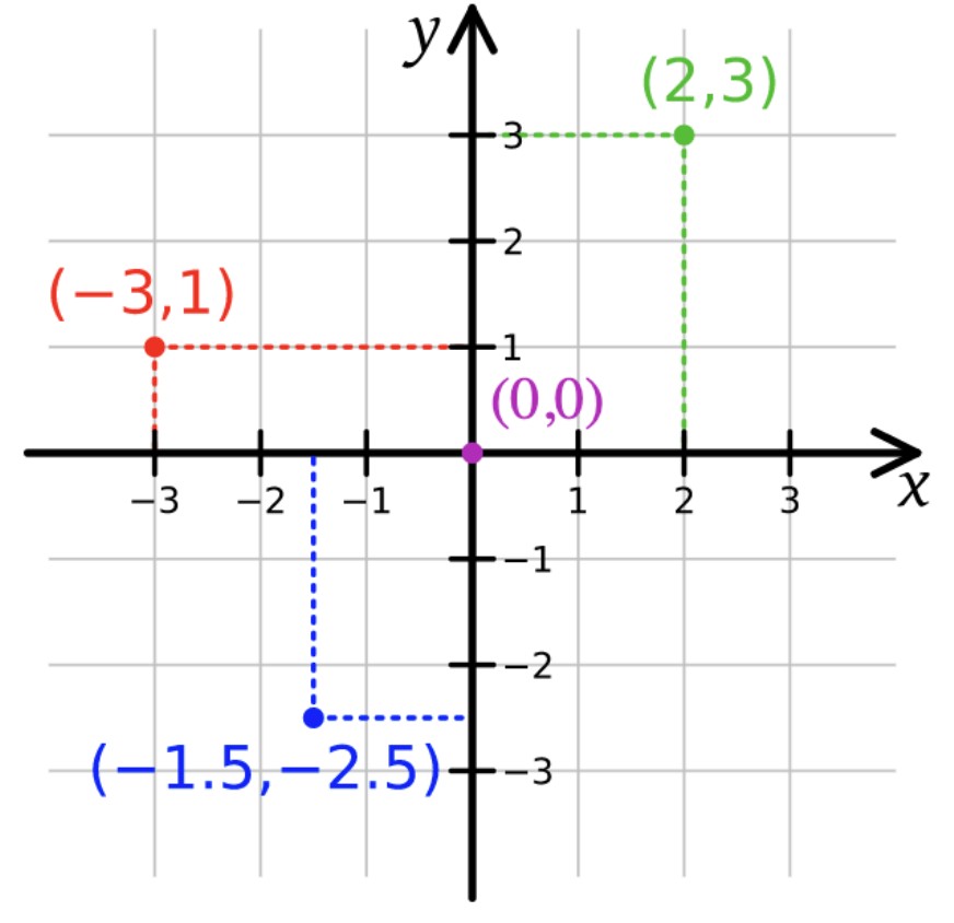
Two-dimensional coordinate system
In that context, we say that a pair of numbers (i.e. [-3, 1] in the figure), is a two-dimensional vector that we use to describe the location of a point. If we consider symbols X and Y to represent any number each, the symbolic vector (X, Y) contains all of the spatial information about any kind of surface. You can map a planet with that knowledge.
Going from 2 to 3 dimensions is just a formality – simply add a third number, Z, changing the symbolic vector into (X, Y, Z). Now you have a tool that can be used to describe any location in a 3-dimensional space. If you want to go further, we recommend the physics way – add a fourth number, T, and now there is a 4-dimensional entity, (X, Y, Z, T) that is basically equivalent to what physicists call a space-time continuum.
Notice that we are increasing both the number of dimensions and number symbols by 1 – this is not a coincidence. For our purposes we can define the number of dimensions of any space/object as the number of coordinates required to represent position.
At this point, you have to diverge from the spatial reality of everyday experience and increase dimensionality by adding symbols/numbers to the vector. For example, to make it 10-dimensional, you could use something like: (X, Y, Z, T, A, B, C, D, E, F). Going after notation simplicity it can be written as (X1, X2, X3, …, X10) or [Xn] for n in [1, 10]. Now we can say that we have a vector describing a space of 10 dimensions – that’s basically all you need to do string theory.
With images we want to know something more than just positions of points on the surface – we want to understand the content contained in the image. The way that computers can handle visual information is by introducing pixels – dividing the picture into a multitude of elements (hence the name ‘pix-els’) each with its color information described by a set of numbers. The most popular set is of course R, G, B. Like we’ve discussed in the previous paragraph, these three symbols represent three dimensions of what we call a “color space”).
So it turns out that pictures are 2-dimensional in terms of physical (geometric) space, but have much higher dimensionality in terms of information content. In fact, we need 5 numbers to fully describe just one pixel: 2 for position and 3 for color.
If we now consider 12 Megapixels (12,000,000 pixels; the average image resolution on an iPhone), we can say that we need 12,000,000 * 5 = 60 million dimensions to precisely describe all of the information contained in that image. This description will allow us to reproduce the image with 100% precision, which technically speaking would be a copy.
Similarity is distance
Now that we have established that images are mathematical objects existing as points in a multi-million-dimensional space, we can start thinking about measuring the visual similarity between any images in that space. Usually, similarity is defined as some kind inverse of distance – low distance equals high similarity.
So all we need to calculate that value is a distance function that is somehow related to the visual content of the image. One straight-forward approach would be to measure the per-pixel difference between images. This approach is simple enough to implement, but the results are not at all impressive. There are other “traditional” (without deep learning) methods, like structural similarity, compare, that might give better outcomes, but that only work properly in a very limited number of cases.
What is distance?
In practice, it is something you can measure. In theory, it is something you can calculate. Measuring distance is pretty straightforward, (as long as there are no black holes in your vicinity) and we all intuitively know what the resulting number is.
Since we are dealing with purely numerical problems, we are not going to be measuring any distance in the physical sense. What we need is to find a function that takes information about two points (a and b) and returns a number that we will call “distance between a and b”. We call a function like that a “metric”, and it turns out that this is a very potent starting point in terms of physics and mathematics that can emerge from it – with the finest example being the general theory of relativity that describes the relationship between mass and distance (as measured in space, time or both).
Reducing 60,000,000 to 500 with neural net vision
Even though we live during the times when data is often called the “new oil”, having that much knowledge about a single picture raises a lot of problems – so much in fact, that scientists working in those areas coined the cheery term “curse of dimensionality” to sum up all of the hurdles of having too much of information. Combine this with a very high computational cost of any kind to process those amounts of data and it turns out that if you want to utilize every bit, you are limited to building solutions that are either very expensive or very slow.
This is a not an uncommon situation and the way out very often turns out to be some kind of dimensionality reduction – which is a generic term for a procedure that will encode the information using fewer bits than the original representation (which is exactly what compression does when all you want to do is save storage space).
The method we will use is based on a representational power of deep neural networks, a technique that was first described in the Alexnet paper. In a very simplified description, you can view multi-layer neural networks as a sequence of steps transforming the input information”
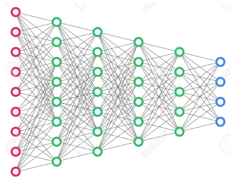
The first layer (red) contains the full information about the input, and the last (blue) just the thing that the network was trained to extract and has a very low number of dimensions compared to the input. In the case of Alexnet paper, they showed that using the second to last layer as a low dimensional description of the input image gives you amazing capabilities for visual similarity assessment:
We are not using the initial millions of dimensions that represent the information content of the image, but rather only 500 dimensions that represent in purely numerical form what a deep neural network perceives on that image. But enough theory.
Next, we’ll show all the necessary steps for building a search engine based on that mechanism in a quick tutorial.
Visual search tutorial
In this tutorial we’ll be using the Flickr 30k dataset: https://www.kaggle.com/hsankesara/flickr-image-dataset
Here’s a Notebook showing how to recreate the results: https://github.com/filestack/visual-search-tutorial
Image based search engines seem to be all the rage right now in the field of applied deep learning. From Amazon to Zalando, tech companies invest resources with the idea of using pictures as a search input, or, visual search. We’re going to demonstrate how to get started with building a search engine for images, based on deep neural network feature vectors.
Feature vectors
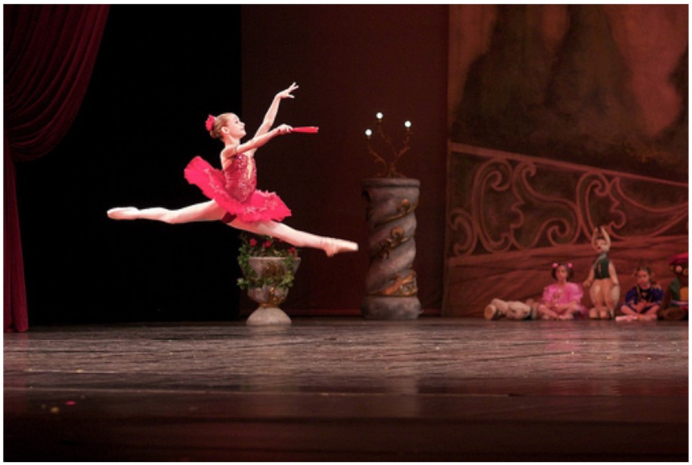
Features of an image, in human terms, are all the things you can say in order to describe a given picture. Let’s look at an example:
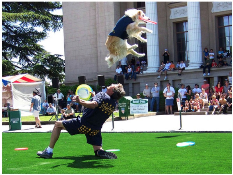
Phrases that come to mind: “dog”, “jump”, “greek columns in the background”, “summer”, “sport” etc. all could be considered features of this image. Unfortunately, working with descriptions like that does not work very well as subject of software processing – undefined length, subjectivity, natural language – these are hard problems for computers to scale and may not be a perfect fit for many possible applications – if you ever had to look for images just using hashtags you probably know the feeling of disappointment that it can give rise to.
For computer vision engineers, features of an image are numeric structures that were generated using that image and designed to represent some property specific to that image. History of visual feature design comprises many impressive solutions, but nothing has had nearly as much impact on progress in visual processing as deep learning and its rise to power during the last couple of years. While training a deep neural network to perform some visual task (e.g. image classification or object detection) as a by-product, you get a system for feature extraction that outperforms everything prior.
One of the use cases for those features is image comparison. In their 2017 paper, Krizhevsky, Sutskever, and Hinton mention a method to measure image similarity as an euclidean distance between vectors of activations induced by an image at the last 4096-dimensional hidden layer. Their model, known as the AlexNet was designed to solve a different task: ImageNet classification of high resolution images into 1000 categories for the LSVRC contest. During research they discovered that intermediate layers can be used as low-dimensional representations of the images.
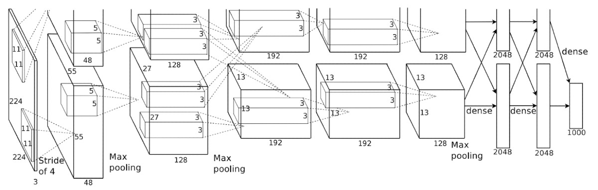
AlexNet original architecture diagram created by the authors. The layer used to extract features is the second to right.
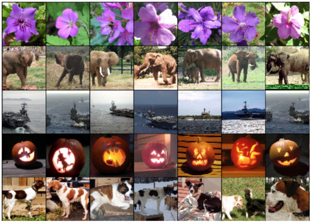
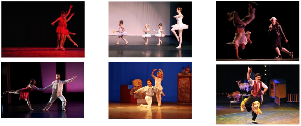
Looking at the output of such a layer as a vector embedded in a 4096-dimensional space, they showed that images that produce a vectors that are closer together in that space exhibit very compelling visual similarity:
The first image on the left is the input image, the following are similar images retrieved from the database.
This is an impressive level of visual similarity and that’s the method we’ll implement. Instead of AlexNet we will use ResNet to have more flexibility in how deep we want our base network.
Using ResNet50 we get a 2048-dimensional feature vector for every image. For the jumping dog shown above we get this:
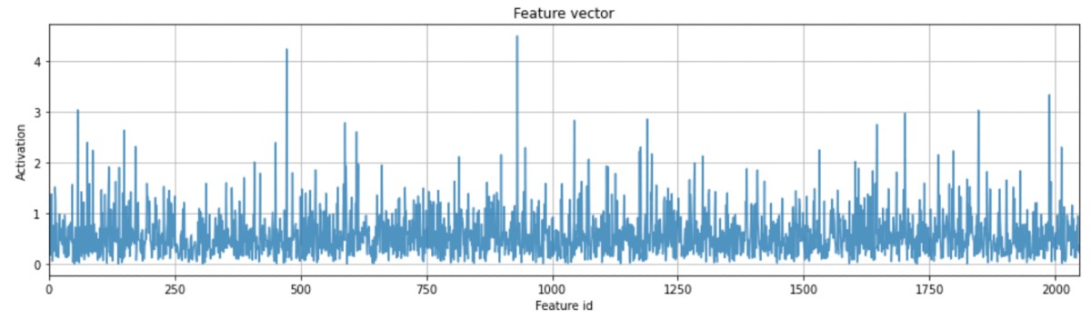
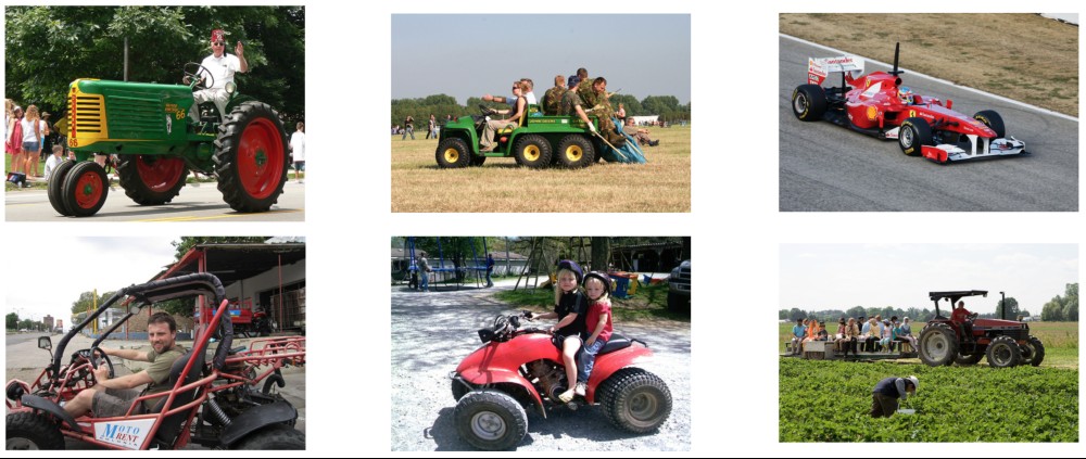
This may seem like noise at first inspection, but if we treat this data as a position in a 2048-dimensional space, we can find a couple of images bearing interesting similarities with the input image (which is mathematically equivalent to being close to the input image in that 2048-dimensional space):
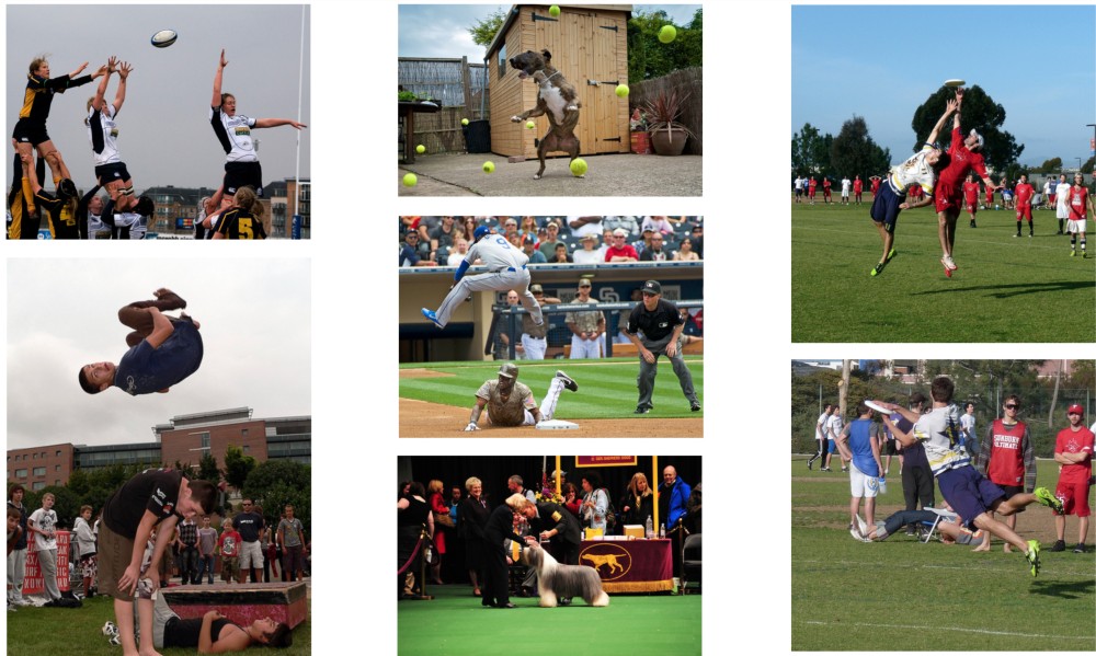
Here are some additional examples of search results for different input images:
Input
Results
Another Input<

Results
Filestack is a dynamic team dedicated to revolutionizing file uploads and management for web and mobile applications. Our user-friendly API seamlessly integrates with major cloud services, offering developers a reliable and efficient file handling experience.
Read More →