The need for color quantization comes from the old days when the hardware needed to display color images was rather slow and expensive. At that time, it wasn’t possible to display color images in 24 bits, 8 bits for each color channel (red, green and blue). Each pixel was typically 8 bits deep, and the need to counteract this limitation was imminent. Color quantization reduces the number of distinct colors of an image while keeping the new image visually similar to the original. For this purpose generally a color table has been enrolled, where a single 8-bit index could be used to specify up to 256 different 24-bit colors.
The mentioned limitations are not an issue thanks to the improvements of hardware technology, however there are certain cases when this technique can be used. For example:
- Certain displays of embedded systems are limited to a low resolution
- Situations where the goal is to reduce the image size while minimizing the perceptual loss in the output quality
Color Quantization Applied Today
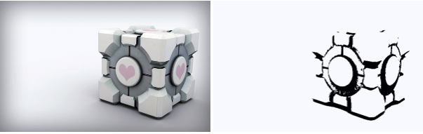
To reiterate, color quantization is trying to reduce the number of distinct colors to a set of representative ones. Even with the best set of 256 colors, there are many images that still might look bad. One of the most common problems are contours around slowly changing color regions. Here is an example showing this issue.
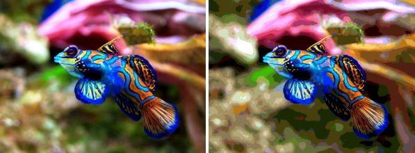
To counteract this kind of limitation, we used a well known image processing method called error diffusion dithering (EDD). Error diffusion dithering works by computing the error between pixel value and its nearest representative; then propagating that error to the nearby pixels that has not yet been assigned to a color in the color map. After applying the error diffusion, the average color of a region is remarkably similar to the average color of the original region, however the individual colors of the resulted image are constrained to be taken from the color table.
There are many error diffusion dithering methods like Atkinson, Burkes, Stucki, Sierra-2, Sierra-3, Sierra-Lite, but the best know is Floyd-Steinberg. All of these algorithms have something in common: they diffuse the error in two dimensions, but they always push the error forward, never backward. The reason for this is obvious: by pushing the error backward we have to revisit every pixels already processed, leading to an infinite cycle of error diffusion.
We can represent this with the following diagram:
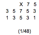
where x represents the current pixel processed. The fraction at the bottom is the divisor for the error. We will come back to this topic shortly.
Quantization Methods
There are a few methods for solving the problem of finding good representatives of colors. The simplest is a fixed size partitioning which covers the entire color space without requiring a first pass over an image to generate the partitioning, but it’s not producing good results. An adaptive color partitioning is doing a much better job, because it requires two steps to generate the color table: on the first pass it gathers the image statistics (where it might not need to sample every pixel in the image) and on the second pass constructs the representative colors. Three types of adaptive color quantification methods have been widely adopted: popularity, median cut and octree. We will focus on the median cut algorithm.
In each of the above mentioned methods the division of the color space can be represented by a tree. Generate the tree either by starting with the entire color space and splitting it up or by taking a large number of small volumes and merging them together. The median cut method uses a splitting algorithm to have a roughly equal distribution of pixels in the resulting volumes. It is implemented by repeatedly splitting the color space (the cluster) with the most pixels up until the desired number of clusters have been populated or when the clusters cannot be further split.
Color Dithering
The goal of color quantization is to generate a color palette of the given image’s most representative colors, or in other terms, to obtain the most dominant colors of an image. This goal does not take visual appeal into account. This is where color dithering proves valuable.
As we mentioned above, dithering is fundamentally about error diffusion. Let’s use a grayscale image as an example. The goal here would be to apply a threshold, i.e. to turn all of the pixels below a certain value black and all of the pixels above that value white. When converting the pixels to halftone images, we use a simple formula: if the pixel value is closer to 0 (pure black) turn it black otherwise turn it white. Take the value 117 as an example: this is closer to 0 (black), so we’ll convert to black. The standard approach would be to simply move to the next pixel and apply the same formula. However, a problem arises when we have a bunch of the same pixels. They are all getting turned black and we are left with a huge bank of black pixels.
Error diffusion takes a more advanced approach: it spreads the error of each calculation to the neighboring pixels. On each step it does not simply apply the same formula to the next pixel, but take note of the previous error and adds the error weight to the current pixel. For example, if the current pixel is still 117, it does not simply convert the pixel color to black, but calculates the new pixel value based on the previous pixel error weight.
The following code is a simple implementation of the above method.
[code lang=”go”]// Dither is a two dimensional slice for storing different dithering methods.
type Dither struct {
Filter [][]float32
}
// Prepopulate a multidimensional slice. We will use this to store the quantization level.
rErr := make([][]float32, dx)
gErr := make([][]float32, dx)
bErr := make([][]float32, dx)
// Diffuse error in two dimension
ydim := len(dither.Filter) – 1
xdim := len(dither.Filter[0]) / 2 // split the X dimension in two halves
for xx := 0; xx < ydim + 1; xx++ {
for yy := -xdim; yy <= xdim – 1; yy++ {
if y + yy < 0 || dy <= y + yy || x + xx < 0 || dx <= x + xx {
continue
}
// Propagate the quantization error
rErr[x+xx][y+yy] += float32(er) * dither.Filter[xx][yy + ydim]
gErr[x+xx][y+yy] += float32(eg) * dither.Filter[xx][yy + ydim]
bErr[x+xx][y+yy] += float32(eb) * dither.Filter[xx][yy + ydim]
}
}[/code]
Then we can plug-in any of the above mentioned dithering methods, just by replacing the two dimensional filter array components with the error propagation values.
For example the Floyd-Steinberg dithering method can be expressed as:
[code lang=”go”]colorquant.Dither{
[][]float32{
[]float32{0.0, 0.0, 0.0, 7.0 / 48.0, 5.0 / 48.0},
[]float32{3.0 / 48.0, 5.0 / 48.0, 7.0 / 48.0, 5.0 / 48.0, 3.0 / 48.0},
[]float32{1.0 / 48.0, 3.0 / 48.0, 5.0 / 48.0, 3.0 / 48.0, 1.0 / 48.0},
}
}[/code]
Color Quantization Use Cases
Applying the error diffusion algorithm on a quantized image results in a smaller (but qualitative) almost imperceptible image, that might greatly improve the performance of a CDN as an example. Color quantization can also be used to obtain the most dominant color of an image, which might be useful in case we wish to apply some custom settings based on the processed image.
Take an e-commerce platform for example. Color quantization could help the e-commerce platform show the products which closest resemble colors requested by customers. The possible applications are endless, and we encourage any questions in the comment section!
Filestack is a dynamic team dedicated to revolutionizing file uploads and management for web and mobile applications. Our user-friendly API seamlessly integrates with major cloud services, offering developers a reliable and efficient file handling experience.
Read More →